CenterNet
참고
Objects as Points
2019
Introduction
기존의 방법과 다르게 object를 bounding box의 중심으로 나타냄
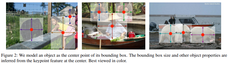
Object 크기, 차원, 3D 확장, 방향, 포즈 등의 속성들의 center location의 특징에서 직접적으로 regression하여 획득
이미지를 fully-connected network의 입력으로 사용하여 heatmap 생성하고, 이 heatmap의 peak는 object의 center를 의미
각 peak에서의 feature는 object bounding box의 height, width를 예측함
모델의 학습은 standard dense supervised learning 으로 진행이되고 추론은 post-processing을 위한 NMS 없이 하나의 network forward-pass로 진행
이런 방법은 일반적이고 그렇기 때문에 다른 task로 쉽게 확장 할 수 있음
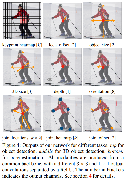
이 논문에서는 각 center point에서 추가적인 output을 예측하여 3D object detection 과 multi-person human pose estimation의 실험 결과를 제시함
우리가 제시하는 방법인 CenterNet은 단순하고 매우 빠른 추론 속도를 가짐
Preliminary
Width가 $W$, height가 $H$ 인 input image를 $I\in R^{W\times H\times 3}$ 로 나타냄
우리의 목표는 keypoint heatmap $\hat{Y}\in [0,1]^{\frac{W}{R}\times \frac{H}{R}\times C }$을 생성 (추정) 하는 것
이 때, $R$은 output stride이고, $C$는 keypoint type의 수
Human pose estimation에서는 joint 수인 $C=17$이고 coco dataset을 이용한 object detection에서는 object의 category 수 (=class 수) 인 $C=80$
Output stride는 $R=4$ 를 default 값으로 사용하고 이를 이용해 output을 downsampling
\(\hat{Y}_{xyc}=1\) 이면 center point, $\hat{Y}_{xyc}=0$ 이면 background 임을 의미
몇 개의 다른 fully-convolutional encoder-decoder network를 이용하여 $\hat{Y}$를 예측
- Stacked hourglass network, Upconvolutional residual networks (ResNet), Deep layer aggregation (DLA)
Keypoint detection network의 학습은 CornerNet 을 따름
Class $c$에 대한 각 ground truth point ($p\in R^{2}$) 가 있을 때, low-resolution equivalent $\tilde{p}=[\frac{p}{R}]$ 을 계산
그 후, 모든 ground point에 Gaussian kernel을 적용하고($Y_{xyc}$) heapmap $Y \in [0, 1]^{\frac{W}{R}\times \frac{H}{R}\times C }$ 을 생성
즉, ground truth에 전처리를 하여 학습이 더 잘 되게 반영
\[Y_{xyc}=exp(-\frac{ (x-\tilde{p}_{x})^{2}+(y-\tilde{p}_{y})^{2} }{2\sigma^{2}_{p}})\]- $\sigma_{p}$ : object size에 adaptive 한 표준 편차
같은 class의 두 Gaussian이 겹치면 element-wise maximum을 계산
Loss 함수는 다음과 같은 focal loss 사용하여 penalty-reduced pixelwise logistic regression
\[L_{k}= \frac{-1}{N}\sum_{xyc} \left\{\begin{aligned} &(1-\hat{Y}_{xyc})^{\alpha}\log(\hat{Y}_{xyc}), \ if \ Y_{xyc}=1 \\ &(1-Y_{xyc})^{\beta}(\hat{Y}_{xyc})^{\alpha}\log(1-\hat{Y}_{xyc}), \ otherwise \end{aligned}\right.\]- $\alpha$, $\beta$ : hyper-parameter
- $N$ : Image $I$ 의 keypoint 수
N 으로 정규화하면 모든 positive focal loss instance를 1이 됨
Output stride로 발생한 discretization error을 헤결하기 위해 각 center point에서 추가적으로 local offset \(\hat{O}\in R^{\frac{W}{R}\times \frac{H}{R}\times C }\) 예측
Center point는 4배 downsampling 된 resolution의 feature에서 에측한 결과이고 이를 다시 input image의 resolution에 대응되게 만들어야 함
모든 class $c$ 들은 같은 offset prediction 공유하고, L1 loss로 학습
\[L_{off}=\frac{1}{N}\sum_{p} |\hat{O}_{\tilde{p}}-(\frac{p}{R}-\tilde{p})|\]Keypoint $\tilde{p}$에 대해서만 supervision acts이 진행이 되고 다른 location에서는 무시됨
Objects as Points
Category $c_{k}$의 object $k$의 bounding box는 \((x_{1}^{(k)}, y_{1}^{(k)}, x_{2}^{(k)}, y_{2}^{(k)})\) 이고, center point $p_{k}$는 \((\frac{x_{1}^{(k)}+x_{2}^{(k)}}{2}, \frac{y_{1}^{(k)}+ y_{2}^{(k)}}{2})\)
Keypoint estimator $\hat{Y}$을 모든 center point를 예측하기 위해 사용
각 Object $k$에 대해서 object size \(s_{k}=(x_{2}^{(k)}-x_{1}^{(k)},y_{2}^{(k)}- y_{1}^{(k)})\)을 regression
계산의 부담을 줄이기 위해, 모든 object category에 대해서 single size에 대한 예측 $\hat{S}\in R^{\frac{W}{R}\times \frac{H}{R}\times C }$ 을 사용
- Low resolution에서 single size에 대하여 예측
L1 loss를 사용하여 학습
\[L_{size}=\frac{1}{N}\sum_{k=1}^{N}|\hat{S_{p_k}}-s_{k}|\]Scale을 normalize 하지 않고 직접적으로 raw pixel coordinate을 사용
전체적인 학습 objective는 아래와 같음
\(L_{det}=L_{k}+\lambda_{size}L_{size}+\lambda_{off}L_{off}\)
Keypoint $\hat{Y}$, offset $\hat{O}$, size $\hat{S}$를 예측하기 위해서 하나의 네트워크를 사용
네트워크는 각 location마다 $C+4$의 output을 가지고 모든 output은 fully-convolutional backbone network를 공유함
From points to bounding boxes
추론 할 때, 우선 각 category에서 독립적으로 heatmap의 peak들을 찾음
값이 8-connected neighbor보다 크거나 같은 모든 response(중간값이라고 생각)를 찾고, 가장 큰 100개의 peak를 저장
$\hat{P}_{c}$는 $n$개의 detection한 class $c$에 대한 center point \(\hat{P}=\{(\hat{x}_{i},\hat{y}_{i}) \}^{n}_{i=1}\)의 집합
각 keypoint location은 정수인 좌표 $(x_{i}, y_{i})$ 로 나타냄
Key point value인 \(\hat{Y}_{x_{i}y_{i}c}\)를 detection confidence를 측정하고, bounding box를 측정하는데 사용
- Heatmap을 이용하여 confidence 측정
Boudning box는 아래와 같이 나타냄
\[(\hat{x}_{i}+\delta\hat{x}_{i}-\hat{w}_{i}/2, \hat{y}_{i}+\delta\hat{y}_{i}-\hat{h}_{i}/2 \\ \hat{x}_{i}+\delta\hat{x}_{i}+\hat{w}_{i}/2, \hat{y}_{i}+\delta\hat{y}_{i}-\hat{h}_{i}/2 ) \\\]- \((\delta\hat{x}_{i}, \delta\hat{y}_{i})=\hat{O}_{\hat{x}_{i},\hat{y}_{i}}\) : offset prediction
- \((\hat{w}_{i}), \hat{h}_{i}=\hat{S}_{\hat{x}_{i}}, \hat{y}_{i}\) : size prediction
모든 output들은 IoU 기반의 NMS 방식을 사용하지 않고 keypoint estimation에서 직접적으로 얻음
Implementation detailsf
4 가지 아키텍쳐에 대하여 실험을 진행
- ResNet-18, ResNet101, DLA-34, Hourglass-104
Hourglass
Stacked Hourglass Network 는 2개의 연속된 hourglass module을 지나면서input을 4배 downsampling
이 네트워크는 크지만, 일반적으로 가장 좋은 keypoint estimation 성능을 도출
ResNet
Simple baseline에서는 standard residual network에 3개의 up-convolution network를 추가하여 higher-resolution output 생성
CenterNet에서는 3개의 upsampling layer의 채널을 각각 256, 128, 64로 바꿈
- 계산량을 줄이기 위해
각 up-convolution layer 전에 하나의 3 $\times$ 3 deformable convolution layer를
추가
Up-convolutoion kernel은 bilinear interpolation으로 초기화
DLA
Deep Layer Aggregation (DLA) 는 hierarchical skip connections을 가지는 image classification network
Dense한 prediction을 위해 DLA의 fully convolutional upsampling 사용
매 upsampling layer에 3$\times$3 deformable convolution을 적용
Experiments
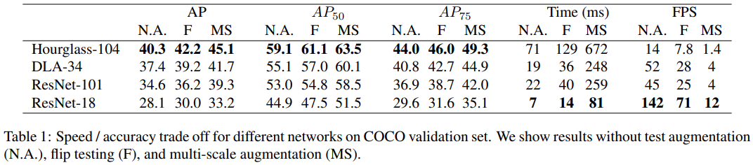
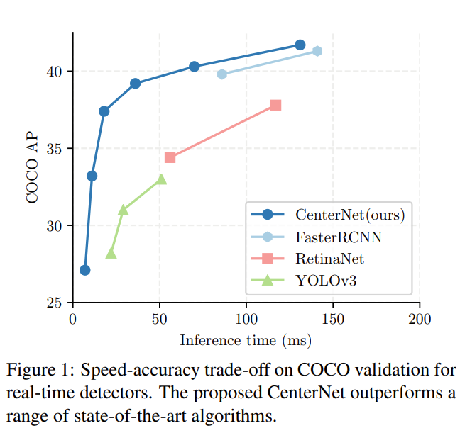
- Hourglass-104가 가장 좋은 성능을 보임을 확인
- 이 때, CornerNet 과 and ExtremeNet 보다 속도와 정확도가 더 좋음을 확인
- ResNet-101
- 같은 backbone RetinaNet 성능 능가
- DLA-34
- 속도와 정확도의 가장 좋은 trade-off 제공
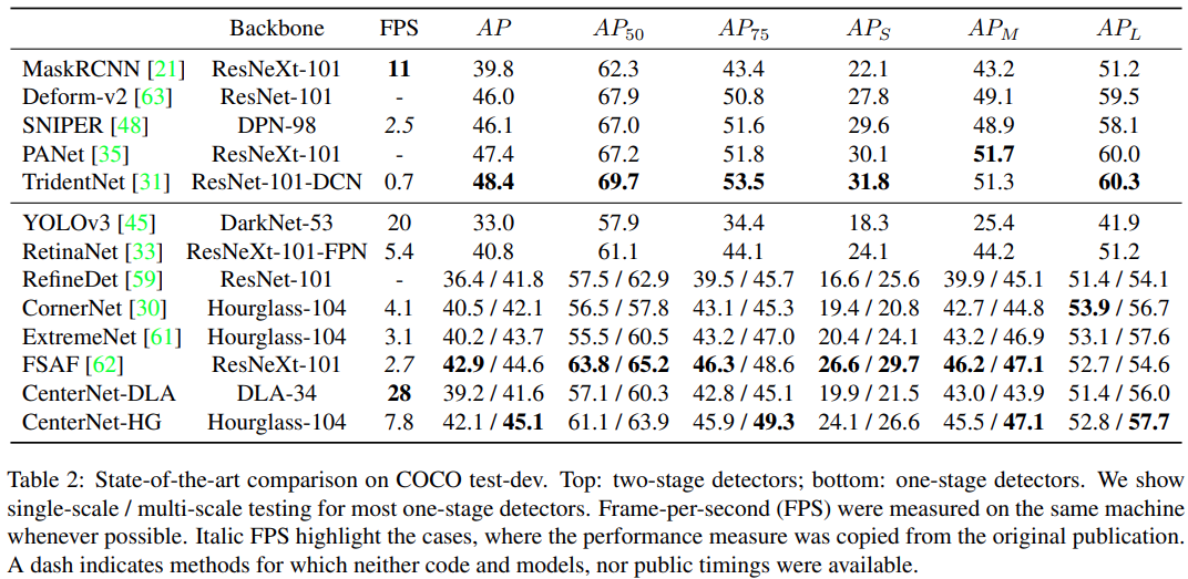
- 2 stage 방법들이 정확도가 더 좋으나, 속도가 느림
- CenterNet과 sliding window detector 방식의 차이가 없음
Conclusion
CenterNet은 keypoint estimation 방법을 통해 성공적으로 object detection을 한 방법
이 알고리즘은 간단하고, 빠르고 정확하며 NMS post-processing 없이 end-to-end로 미분 가능
2차원 object detection 뿐만이 아니라 다른 task에도 확장 가능