Point Cloud 특징 추출 방법
참고
- https://pcl.readthedocs.io/projects/tutorials/en/latest/pfh_estimation.html
- https://pcl.readthedocs.io/projects/tutorials/en/latest/fpfh_estimation.html
- https://velog.io/@intuition/LiDAR-3D-object-detection-3-LaserNet-An-Efficient-Probabilistic-3D-Object-Detector-for-Autonomous-Driving
- https://robotica.unileon.es/index.php?title=PCL/OpenNI_tutorial_4:3D_object_recognition%28descriptors%29
Point Cloud 특징 추출
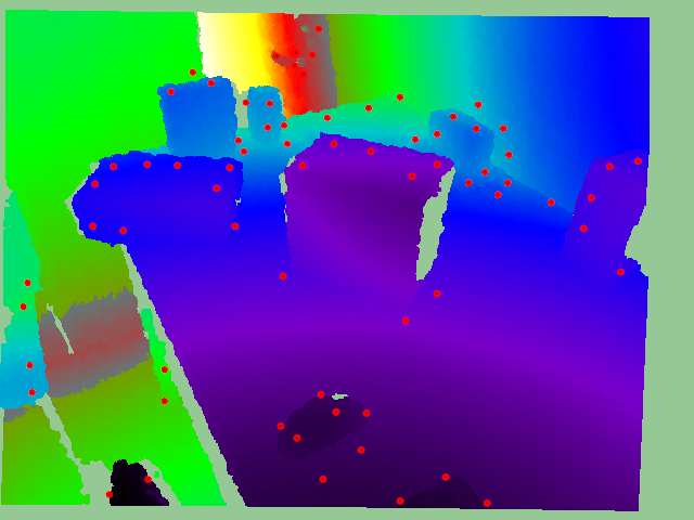
Harris corner 3D
Harris corner는 Computer vision에서 corner point, interest region 찾을 대 가장 기본적으로 사용하는 방법
이 방법을 3D로 확장한 방법
\[E(u, v, w)=\sum_{x,y,z\in \Omega}{[I(x+u, y+v, z+w)-I(x,y,z)]^{2}}\\\]위 식에서 window function 생략됨
\[E(u,v,w)\approx \begin{bmatrix} u& v& w\end{bmatrix}\ M \ \begin{bmatrix}u\\ v\\ w \end{bmatrix}\] \[M=\sum_{x,y,z\in \Omega}\begin{bmatrix} I_{x}^{2} &I_{x}I_{y} &I_{x}I_{z}\\ I_{y}I_{x} &I_{y}^{2} &I_{y}I_{z}\\ I_{z}I_{x} &I_{z}I_{y} &I_{z}^{2} \end{bmatrix}\]Harris corner 6D
x, y, z의 intensity 뿐만이 아니라 normal vector 정보를 추가하여 정확한 특징 값을 찾도록 함
ISS (Intrinsic Shape Signatures)
Covariance matrix 정의하고, 이를 기반으로 Eigenvalue Decomposition 진행하여 $\lambda_{1}$,$\lambda_{2}$,$ \lambda_{3} $ 찾음
- $\lambda_{1}$ > $\lambda_{2}$ > $\lambda_{3}$
그리고 point에 대하여 아래의 두 조건을 만족하는 signature feature 찾음
\[\frac{\lambda_{2}(p)}{\lambda_{1}(p)} < \gamma_{12}\] \[\frac{\lambda_{3}(p)}{\lambda_{2}(p)} < \gamma_{23}\]PFH (Point Feature Histogram)
Histogram을 기반으로 point cloud 특징을 검출하는 descriptor
아래과 같은 순서로 진행
-
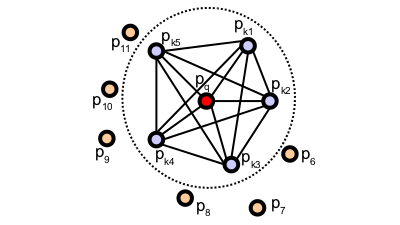
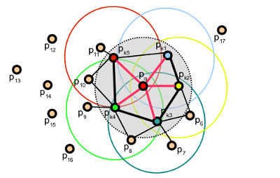
특징을 뽑고자 하는 $p_{q}$ point에 특정 반경 $r$ 만큼의 neighborhood 선택
출처 -
$p_{q}$와 모든 neighborhood들의 connection을 연결하여 pair를 만듦
-
각 pair point들의 normal vector와 구해진 normal vector를 이용하여 위의 그림처럼 고정된 uvw 좌표 프레임 정의
출처 -
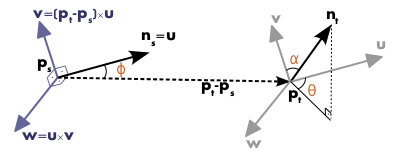
PCA 알고리즘을 사용하여 normal vector $n_{i}$, $n_{j}$를 구함
-
구해진 normal vector를 이용하여 위의 그림처럼 고정된 좌표 프레임을 정의 (uvw 프레임)
\[\begin{align} u&=n_{s}\\ v&=u\times \frac{(p_{t}-p{s})}{||p_{t}-p_{s}||_{2}} \\ w &= u\times v \end{align}\]
-
-
3에서 구한 값을 바탕으로 $f_{1}$, $f_{2}$, $f_{3}$, $f_{4}$ 계산
\[\begin{align} f_{1}&=v \cdot n_{t}\\ f_{2}&=||p_{t}-p_{s}|| \\ f_{3}&=u\cdot (p_{t}-p_{s})/f_{2}\\ f_{4}&=atan(w\cdot n_{t}, u\cdot n_{t}) \end{align}\] -
$f_{1} $ ~ $f_{4}$ 을 이용하여 indexing
\[idx=\sum_{i=1}^{i\leq 4}step(s_{i},f_{i})\cdot2^{i-1}\]- $s_{i}$ 값보다 $f_{i}$ 값이 크거나 같으면 1, 아니면 0
- 0부터 15까지의 값을 가짐
-
Index 값을 이용하여 16개의 bin을 가짐 histogram 을 기반으로 descriptor 생성
FPFH (Fast Point Feature Histogram)
PFH는 특정 범위 안의 모든 point들의 pair에 대하여 계산한다는 단점 존재
이 문제를 해결하기 위해서 나온 방법
https://zzziito.tistory.com/m/47 참고하여 정리…
NARF (Normal Align Radial Feature)
Normal 값을 적극적으로 활용하고 있는 방법론
-
Point Cloud를 range 이미지로 변환
- Range 이미지는 다음에 정리 예정
-
Range 이미지를 이용하여 물체의 경계 찾음
출처 -
찾은 경계 point로부터 normal vector 계산
-
경계가 아닌 곳에서 주 곡률 계산
-
곡률 기반으로 하여 모든 점들에 대한 특이점 (Interest point) 계산
-
Keypoint 분리
출처 -
각 point에 대한 descriptor 계산
표면이 안정적이고, 근처에 주요 변화가 명백하게 있는 영역에서 NARF 사용하면 keypoint를 조금 더 정확하게 계산할수 있고 도드라지게 찾아낼 수 있음
비연속적인 변환으로 발생하는 edge 집중적으로 보면서 고려할 수 있는 방법론